Material Balance Introduction

The material balance equation is one of the fundamental equations a reservoir engineer needs to understand. Some of it’s applications include the following:

Determining the initial hydrocarbon in place
Predicting an overall recovery factor
Determining reservoir drive mechanisms

The material balance equation can be intimidating for someone looking at it for the first time. It was for me, but it is really not too bad if you understand the basic concepts behind it. Material balance simply compares the original volumes at initial reservoir pressure to the current volumes at a lower pressure. It is zero dimensional, meaning that it compares the initial state to the current state and nothing else. The concept of material balance is easy to understand if viewed as an expanding piston. A conceptual view of material balance is presented in the figure below:

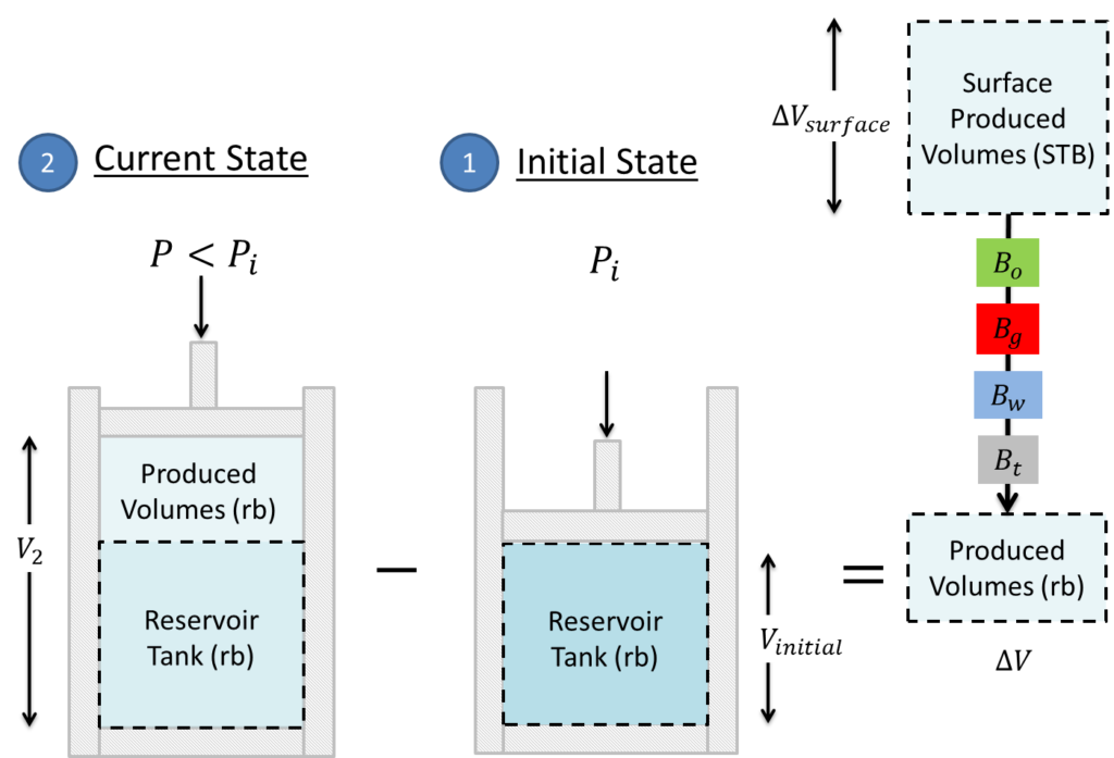
From the figure above it is clear that the fluids expand in the reservoir at a lower pressure. In the material balance approximation, the expanded volumes are the produced volumes. Some key points that can be observed from the figure above are the following:

The difference between the volume at a lower pressure ( $V_2$ ) and the original volume ( $V_{initial}$ ) is equal to the produced volume ( $\triangle V$ )
The volumes we compare in the material balance equation are always in reservoir barrels (rb)
We can convert the surface volumes to reservoir barrels using volume factors
The produced volumes is equal to the expanded fluid volumes ( $\triangle V$ )
We only compare two states: 1) the initial state and 2) any state at a lower pressure

Keep in mind that the material balance process is nothing more than the isothermal compressibility equation discussed previously $(\triangle V = V_i c \triangle P)$ . However, a more convenient form is one that includes surface volumes. The illustration below shows how the compressibility equation can be manipulated to include surface volumes.

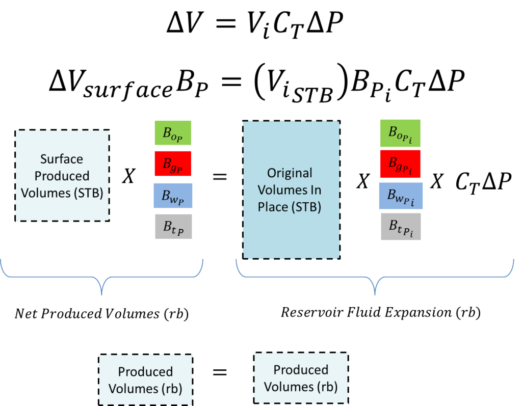
All we did to relate the surface volumes to the reservoir volumes was through a multiple known as the volume factor at their respective pressures. The term on the left hand side represents the net produced volumes in reservoir barrels and the term on the right hand side represents the reservoir fluid expansion in reservoir barrels. If you understand this concept, you will definitely understand the long-winded material balance equation. Without further ado the macroscopic material balance equation is given below:

I know. It’s intimidating. But that is only because it contains additional terms and multiple fluids. I am not going to explain all the terms here, however if you can relate the equation to the compressiblity figure above, you will be golden. The left hand side of the equation is simply the surface produced volumes scaled down to reservoir barrels for each fluid $(\triangle V_{surface} B_P$ ). The right hand side is the reservoir expansion of the original volume in place of each fluid from initial pressure to the current pressure $(V_{i_{STB}}B_{P_i}c\triangle P)$ . It also includes a couple of additional terms, but if you can understand the fluid terms (oil, gas, and water), you will be fine. I’m hopeful this was clear. That’s a wrap!

Nomenclature

$B_g = \text{gas formation volume factor, rb/scf}$
$B_g = \text{initial gas formation volume factor, rb/scf}$
$B_o = \text{oil formation volume factor, rb/stb}$
$B_{to} = \text{two phase oil formation volume factor, rb/stb}$
$B_{to} = \text{initial two phase oil formation volume factor, rb/stb}$
$B_w = \text{water formation volume factor, rb/stb}$
$c_f = \text{pore compressibility, psia}^{-1}$
$G_p = \text{cumulative gas produced, scf}$
$G_I = \text{Gas injected, scf}$
$G_i = \text{initial free gas, scf}$
$N_i = \text{initial oil in place, stb}$
$N_p = \text{cumulative oil produced, stb}$
$P_i = \text{initial reservoir pressure, psia}$
$P = \text{current reservoir pressure, psia}$
$R_v = \text{volatilized oil-gas ratio, stb/scf}$
$R_s = \text{solution gas oil ratio, scf/stb}$
$W_e = \text{cumulative water influx from the aquifer, stb}$
$W_p = \text{cumulative water produced, stb}$
$W_I = \text{injection water, stb}$
$W_i = \text{initial connate water, stb}$
$V_f = \text{total pore volume, rb}$