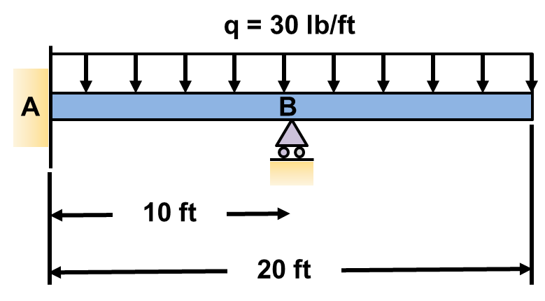
Indeterminate Beam Structures to the First Degree

A beam is considered indeterminate if there a more unknowns than equilibrium equations. When this occurs, one can feel at a loss at what to do or how to proceed. But it really is simple and I am going to provide an example to show you how easy it is. We often classify indeterminate beams based on the difference between the number of unknowns and number of equilibrium equations. For simple static 2-D problems, we always have three equilibrium equations. If we subtract the number of unknowns by the three equilibrium equations, we are left with a number defined as the degree of indeterminacy. For our example we will look at a 1st degree indeterminate beam and explain how to solve it in simple steps. This method can be extended to 2nd, 3rd, and up to n degree indeterminate beam problems. Consider the indeterminate beam below. Solve for the reaction forces:

STEP 1: Draw a FBD and determine the degree of indeterminacy

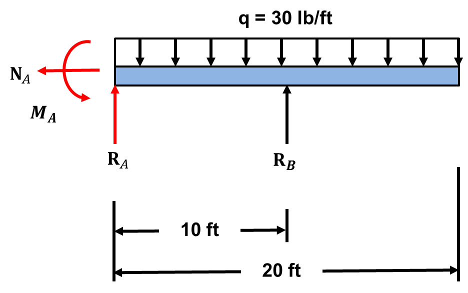
We have 4 unknowns and 3 equilibrium equations. The degree of indeterminacy $= 4-3=1$ . Thus the beam is indeterminate to the first degree and has one redundant support. The degree of indeterminacy tells us how many equations of compatibility we will need to develop to solve the problem. If one does not know what this is, don’t worry we will cover it shortly.

STEP2: Release a redundant support and solve for the deflection at each redundant support location using the beam equations and superposition

The figure illustrates the method of superpostion:

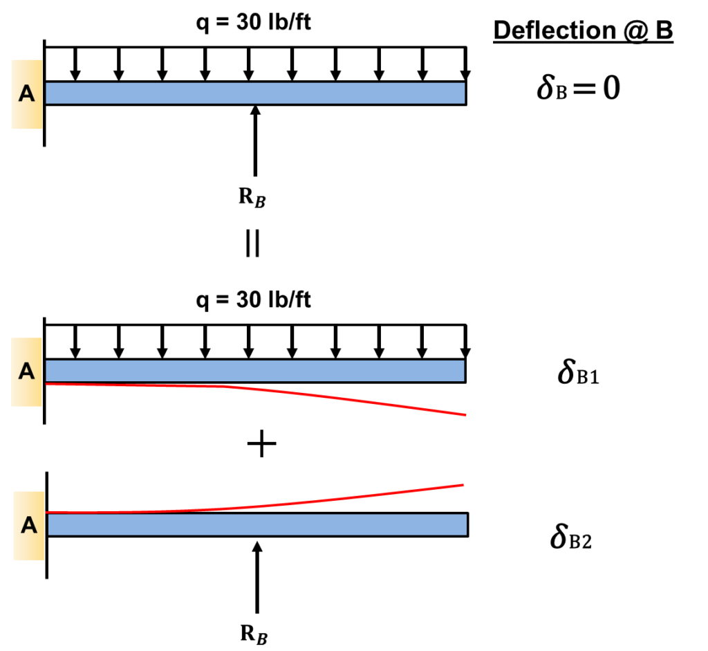
Essentially what your trying to do is divide the beam into load cases that can be solved with beam tables. You then acquire the deflection equations for each load case and solve for the deflections at the redundant supports that one removes. Using beam tables, I was able to locate the correct formulas and solve for the deflections. One can find beam tables in a textbook or online. I used the beam table from OU ecourses website. As always, the proper sign convention must be followed. In this example, I chose an upward deflection as positive, and downward deflection as negative. The results are presented below:

$\begin{align*}\label{Step2}\delta_{B1} &= -\frac{qx^2}{24EI} (6L^2-4Lx+x^2)\\&=-\frac{(30)(10)^2}{24EI}[6(20)^2-4(20)(10)+10^2]\\ &=-\frac{1}{EI}(212,500)\\\\\delta_{B2} &= -\frac{Px^2}{6EI} (3L-x)\\&=\frac{R_{B}(10)^2}{6EI}[3(20)-10]\\&=\frac{1}{EI}(833.33R_{B})\end{align*}$

STEP 3: Apply the compatibility equation at each redundant support location

The compatibility equations provides us with the extra equations we need to solve indeterminate problems. It is essentially is an equation that relates the total deflection at a certain point to the deflections caused by different loads. For simplicity, we usually assume the support is rigid and does not deflect. This simplifies the analysis a lot because we can add up all the deflections and set them equal to zero as shown below using the compatibility equation:

$\begin{align*}\label{Step3}0&=\delta_{B1} + \delta_{B2}\\&=\frac{1}{EI}[-212,500+833.33R_{B}]\\ &R_B=255\, lb\\\end{align*}$

STEP 4: Apply the equilibrium equations to solve for the remaining unknowns

$\begin{align*}\label{Step4}\sum F_x&=0 = N_A\\&N_A=0\, lb\\\\\sum F_y&=0 = R_b -q(20)+R_A\\&0=255-(30)(20)+R_A\\ &R_A=345\, lb\\\\\overset{\curvearrowleft}{+} \sum{M_A} &= 0\\ 0&=-q(20)(10) +R_B(10) + M_A\\0&= -(30)(20)(10) + (255)(10) +M_A\\M_A&=3,450 \,lb\cdot ft\\\end{align*}$

In summary, a step by step method for solving a indeterminant problem to the first degree was presented. The key point is to apply the compatibility equation to solve for the redundant support reactions. Then one can solve for the remaining reactions with the equilibrium equations.